Back to basics - SQL joins

Posted Jul 31, 2019 Updated Oct 13, 2025

By thedarkside.py

12 min read

This tutorial uses Oracle SQL syntax but the concepts are universal.

Joins are the heart of relational databases — they let you combine information stored in different tables into one coherent result. Instead of keeping everything in a single massive table, databases split data into logical chunks (like customers, orders, or products), and joins are how you connect those pieces back together to answer real-world questions. Whether you’re pulling reports, exploring relationships, or building analytics pipelines, mastering joins is what turns raw tables into insight.

INNER JOIN with common key column name

Let’s start with a simple example. Create two sample tables:

  
CREATE TABLE left_table
  (
     id  NUMBER(10) NOT NULL,
     left_val VARCHAR2(50),
     CONSTRAINT left_table_pk PRIMARY KEY (id)
  );

INSERT INTO left_table VALUES (1, 'LEFT 1');

INSERT INTO left_table VALUES (2, 'LEFT 2');

INSERT INTO left_table VALUES (3, 'LEFT 3');

INSERT INTO left_table VALUES (4, 'LEFT 4');

SELECT *
FROM   left_table;

Output:

ID	LEFT_VAL
1	LEFT 1
2	LEFT 2
3	LEFT 3
4	LEFT 4

  
CREATE TABLE right_table
  (
     id  NUMBER(10) NOT NULL,
     right_val VARCHAR2(50),
     CONSTRAINT right_table_pk PRIMARY KEY (id)
  );

INSERT INTO right_table VALUES (1, 'RIGHT 1');

INSERT INTO right_table VALUES (4, 'RIGHT 4');  

INSERT INTO right_table VALUES (5, 'RIGHT 5');

INSERT INTO right_table VALUES (6, 'RIGHT 6');

SELECT *
FROM   right_table;

Output:

ID	RIGHT_VAL
1	RIGHT 1
4	RIGHT 4
5	RIGHT 5
6	RIGHT 6

An INNER JOIN is the default type of join in SQL. It combines rows from two tables based on matching values in a common column. The result only includes rows where a match exists in both tables.

In this case, only ID 1 and 4 appear in both tables.

  
SELECT *
FROM   left_table l
       INNER JOIN right_table r
               ON l.id = r.id

Output:

ID	LEFT_VAL	ID	RIGHT_VAL
1	LEFT 1	1	RIGHT 1
4	LEFT 4	4	RIGHT 4

Note the use of l and r aliases – they make the query easier to read. Since both tables share a column named ID, it appears twice in the result. To tidy things up, we can select specific columns:

  
SELECT l.id,
       left_val,
       right_val
FROM   left_table l
       INNER JOIN right_table r
               ON l.id = r.id

Output:

ID	LEFT_VAL	RIGHT_VAL
1	LEFT 1	RIGHT 1
4	LEFT 4	RIGHT 4

Another way to write an inner join is with the USING keyword, which is handy when both tables share a column with the same name.

  
SELECT *
FROM   left_table l
       INNER JOIN right_table r
USING (id);

The USING keyword works with all standard join types — INNER JOIN, LEFT JOIN, RIGHT JOIN, and FULL OUTER JOIN.

INNER JOIN with different key column names

Let’s look at a case where the key columns have different names.

  
DROP TABLE left_table;

CREATE TABLE left_table
  (
     left_id  NUMBER(10) NOT NULL,
     left_val VARCHAR2(50),
     CONSTRAINT left_table_pk PRIMARY KEY (left_id)
  );

INSERT INTO left_table VALUES (1, 'LEFT 1');

INSERT INTO left_table VALUES (2, 'LEFT 2');

INSERT INTO left_table VALUES (3, 'LEFT 3');

INSERT INTO left_table VALUES (4, 'LEFT 4');

SELECT *
FROM   left_table;

Output:

LEFT_ID	LEFT_VAL
1	LEFT 1
2	LEFT 2
3	LEFT 3
4	LEFT 4

  
DROP TABLE right_table;

CREATE TABLE right_table
  (
     right_id  NUMBER(10) NOT NULL,
     right_val VARCHAR2(50),
     CONSTRAINT right_table_pk PRIMARY KEY (right_id)
  );

INSERT INTO right_table VALUES (1, 'RIGHT 1');

INSERT INTO right_table VALUES (4, 'RIGHT 4');

INSERT INTO right_table VALUES (5, 'RIGHT 5');

INSERT INTO right_table VALUES (6, 'RIGHT 6');

SELECT *
FROM   right_table;

Output:

RIGHT_ID	RIGHT_VAL
1	RIGHT 1
4	RIGHT 4
5	RIGHT 5
6	RIGHT 6

Now the join condition must explicitly match the two differently named columns:

  
SELECT *
FROM   left_table l
       INNER JOIN right_table r
               ON l.left_id = r.right_id

Output:

LEFT_ID	LEFT_VAL	RIGHT_ID	RIGHT_VAL
1	LEFT 1	1	RIGHT 1
4	LEFT 4	4	RIGHT 4

Joins aren’t limited to two tables — you can chain several together to explore more complex relationships.

  
CREATE TABLE another_table
  (
     another_id  NUMBER(10) NOT NULL,
     another_val VARCHAR2(50),
     CONSTRAINT another_table_pk PRIMARY KEY (another_id)
  );

INSERT INTO another_table VALUES (1, 'ANOTHER 1');

INSERT INTO another_table VALUES (3, 'ANOTHER 3');

INSERT INTO another_table VALUES (5, 'ANOTHER 5');

INSERT INTO another_table VALUES (7, 'ANOTHER 7');

SELECT *
FROM   another_table;

Output:

ANOTHER_ID	ANOTHER_VAL
1	ANOTHER 1
3	ANOTHER 3
5	ANOTHER 5
7	ANOTHER 7

Only ID = 1 appears in all three tables, so that’s the only record returned when joining them all:

  
SELECT left_id,
       left_val,
       right_val,
       another_val
FROM   left_table l
       INNER JOIN right_table r
               ON l.left_id = r.right_id
       INNER JOIN another_table a
               ON l.left_id = a.another_id

Output:

LEFT_ID	LEFT_VAL	RIGHT_VAL	ANOTHER_VAL
1	LEFT 1	RIGHT 1	ANOTHER 1

Self join

A self-join is simply a table joined to itself. It’s especially useful for hierarchical or parent-child relationships, such as employees and their managers.

  
CREATE TABLE company
  (
     employee_id   NUMBER(3),
     employee_name VARCHAR(50),
     manager_id    NUMBER(3)
  );

INSERT INTO company
VALUES      (200, 'Mark', NULL);

INSERT INTO company
VALUES      (205, 'Fred', 200);

INSERT INTO company
VALUES      (207, 'Peter', 200);

INSERT INTO company
VALUES      (210, 'Anna', 207);

SELECT *
FROM   company;

Output:

EMPLOYEE_ID	EMPLOYEE_NAME	MANAGER_ID
200	Mark
205	Fred	200
207	Peter	200
210	Anna	207

Using a self join, we can pair each employee with their manager’s name:

  
SELECT c1.employee_id,
       c1.employee_name,
       c1.manager_id,
       c2.employee_name AS manager_name
FROM   company c1
       INNER JOIN company c2
               ON c1.manager_id = c2.employee_id;

Output:

EMPLOYEE_ID	EMPLOYEE_NAME	MANAGER_ID	MANAGER_NAME
205	Fred	200	Mark
207	Peter	200	Mark
210	Anna	207	Peter

LEFT JOIN & RIGHT JOIN

After inner joins, the next family of joins expands the result set.

A LEFT JOIN returns all records from the left table, including those without matches in the right table.

  
SELECT *
FROM   left_table l
       LEFT JOIN right_table r
              ON l.left_id = r.right_id

Output:

LEFT_ID	LEFT_VAL	RIGHT_ID	RIGHT_VAL
1	LEFT 1	1	RIGHT 1
4	LEFT 4	4	RIGHT 4
2	LEFT 2
3	LEFT 3

A RIGHT JOIN does the opposite — it returns all records from the right table, even those without matches in the left. Right joins are less common but work exactly the same way:

  
SELECT *
FROM   left_table l
       RIGHT JOIN right_table r
               ON l.left_id = r.right_id

Output:

LEFT_ID	LEFT_VAL	RIGHT_ID	RIGHT_VAL
1	LEFT 1	1	RIGHT 1
4	LEFT 4	4	RIGHT 4
		6	RIGHT 6
		5	RIGHT 5

FULL OUTER JOIN

A FULL OUTER JOIN combines the results of both left and right joins. It returns all records from both tables, whether or not a match exists.

  
SELECT *
FROM   left_table l
       FULL OUTER JOIN right_table r
                    ON l.left_id = r.right_id

Output:

LEFT_ID	LEFT_VAL	RIGHT_ID	RIGHT_VAL
1	LEFT 1	1	RIGHT 1
4	LEFT 4	4	RIGHT 4
		5	RIGHT 5
		6	RIGHT 6
2	LEFT 2
3	LEFT 3

Note that the order of tables in a query matters. If we switch their order, the output is slightly different.

  
SELECT *
FROM   right_table r
       FULL OUTER JOIN left_table l
                    ON l.left_id = r.right_id

Output:

RIGHT_ID	RIGHT_VAL	LEFT_ID	LEFT_VAL
1	RIGHT 1	1	LEFT 1
		2	LEFT 2
		3	LEFT 3
4	RIGHT 4	4	LEFT 4
6	RIGHT 6
5	RIGHT 5

Note: Some modern databases, like SQLite, don’t support FULL OUTER JOIN directly. You can emulate it using a UNION of left and right joins.

CROSS JOIN

A CROSS JOIN creates all possible combinations of rows from both tables. If one table has x rows and the other has y, the result contains x × y rows. This is also called a Cartesian product.

  
SELECT *
FROM   right_table
       CROSS JOIN left_table

Output:

RIGHT_ID	RIGHT_VAL	LEFT_ID	LEFT_VAL
1	RIGHT 1	1	LEFT 1
1	RIGHT 1	2	LEFT 2
1	RIGHT 1	3	LEFT 3
1	RIGHT 1	4	LEFT 4
4	RIGHT 4	1	LEFT 1
4	RIGHT 4	2	LEFT 2
4	RIGHT 4	3	LEFT 3
4	RIGHT 4	4	LEFT 4
5	RIGHT 5	1	LEFT 1
5	RIGHT 5	2	LEFT 2
5	RIGHT 5	3	LEFT 3
5	RIGHT 5	4	LEFT 4
6	RIGHT 6	1	LEFT 1
6	RIGHT 6	2	LEFT 2
6	RIGHT 6	3	LEFT 3
6	RIGHT 6	4	LEFT 4

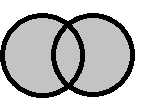
Venn diagrams & set operations

Beyond joins, SQL also supports set operations, which merge results from multiple queries rather than individual rows. Each circle in a Venn diagram represents one result set, and the shading shows which rows are included.

UNION returns all distinct records from both tables.

  
SELECT left_id
FROM   left_table
UNION
SELECT right_id
FROM   right_table

Output:

LEFT_ID
1
2
3
4
5
6

UNION ALL includes duplicates:

  
SELECT left_id
FROM   left_table
UNION ALL
SELECT right_id
FROM   right_table

Output:

LEFT_ID
1
2
3
4
1
4
5
6

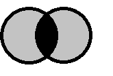
INTERSECT returns only records present in both tables.

  
SELECT left_id
FROM   left_table
INTERSECT
SELECT right_id
FROM   right_table

Output:

LEFT_ID
1
4

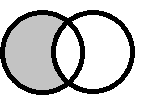
MINUS (or EXCEPT in some databases) returns rows in one table that don’t appear in the other.

  
SELECT left_id
FROM   left_table
MINUS
SELECT right_id
FROM   right_table

Output:

LEFT_ID
2
3

The fields included in all the above operations must be of the same data type, since the results from both queries are stacked on top of each other in the final output.

Semi-joins & anti-joins

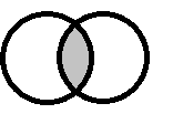
A semi-join returns rows from one table that have matching rows in another, but only shows columns from the first table.

  
SELECT left_id
FROM   left_table
WHERE  left_id IN (SELECT right_id
                   FROM   right_table)

Output:

LEFT_ID
1
4

An anti-join does the opposite — it returns rows that don’t have a match.

  
SELECT left_id
FROM   left_table
WHERE  left_id NOT IN (SELECT right_id
                   FROM   right_table)

Output:

LEFT_ID
2
3

These types of joins don’t have a dedicated SQL keyword like INNER or OUTER JOIN. Instead, they act as filtering mechanisms — limiting rows from one table based on the presence (or absence) of related rows in another.

Subqueries (nested queries)

A subquery (also known as an inner query or inner select) is a query nested inside another query. It can appear in the WHERE, SELECT, or FROM clause. The inner query runs first, and its result feeds into the outer one.

Subqueries don’t have a special syntax — they’re simply regular queries placed inside parentheses within a larger query (often called the outer query or outer select). The database executes the inner query first and then passes its result to the outer query. You can use comparison operators such as >, <, or = to compare this result with another expression.

Subquery inside `WHERE` clause

This is the most common use of a subquery — filtering rows in one table based on values calculated from another.

In the example below, the inner query finds the maximum left_id value from the left_table. The outer query then returns all rows from the right_table where right_id is greater than that maximum value.

  
SELECT *
FROM   right_table
WHERE  right_id > (SELECT MAX(left_id)
                   FROM   left_table)

Output:

RIGHT_ID	RIGHT_VAL
5	RIGHT 5
6	RIGHT 6

Subquery inside `SELECT` clause

Here, the subquery acts like a calculated column. For each row in the outer query, the inner query runs once and produces a value that becomes part of the result set.

In this case, the inner query counts how many times each right_id appears in the left_table. The result is shown in a new column called left_id_count.

  
SELECT DISTINCT right_id,
                (SELECT COUNT(*)
                 FROM   left_table
                 WHERE  left_table.left_id = right_table.right_id) AS
                left_id_count
FROM right_table  

Output:

RIGHT_ID	LEFT_ID_COUNT
1	1
4	1
5	0
6	0

In other words: “For every row in the right table, count how many matching rows exist in the left table.”

Subquery inside `FROM` clause

When a subquery appears in the FROM clause, it behaves like a temporary table or derived dataset that the outer query can reference.

In this example, the inner query calculates the maximum left_id value from the left_table and labels it as left_max_id. The outer query then joins that single-row result to the right_table and retrieves any matching IDs.

  
SELECT right_table.right_id,
       subquery1.left_max_id
FROM   right_table,
       (SELECT MAX(left_id) AS left_max_id
        FROM   left_table) subquery1
WHERE  subquery1.left_max_id = right_table.right_id;

Output:

RIGHT_ID	LEFT_MAX_ID
4	4

Effectively: “Find the maximum ID in the left table, then show any rows from the right table that share that same ID.”

Quick summary

There are six primary SQL joins:

INNER JOIN (including self-joins)
LEFT JOIN, RIGHT JOIN, and FULL OUTER JOIN
CROSS JOIN

You can also combine data using set operations (UNION, UNION ALL, INTERSECT, EXCEPT) and refine it with subqueries in the WHERE, SELECT, or FROM clause.

Conclusion

SQL joins are fundamental to working with relational data. They allow you to combine information from multiple tables to answer complex questions efficiently. Whether for analysis, reporting, or engineering, a solid grasp of join logic is essential in everyday data work.

Tutorials

SQL DatabaseFundamentals

This post is licensed under CC BY 4.0 by the author.

INNER JOIN with common key column name

INNER JOIN with different key column names

Self join

LEFT JOIN & RIGHT JOIN

FULL OUTER JOIN

CROSS JOIN

Venn diagrams & set operations

Semi-joins & anti-joins

Subqueries (nested queries)

Subquery inside WHERE clause

Subquery inside SELECT clause

Subquery inside FROM clause

Quick summary

Conclusion

Trending Tags

Subquery inside `WHERE` clause

Subquery inside `SELECT` clause

Subquery inside `FROM` clause